Keep cart position and rod angle in the same loop
The upright rod is unstable, so correcting angle alone can send the cart down the track. The documented apparatus used a cable-driven DC motor, two potentiometers and end-of-track switches. Position and rod angle were measured; cart velocity and angular velocity were calculated. All four states contribute to one motor command.
Connect the saved calibration to a stated model
The surviving workbook records a 1.021 kg cart, a 0.65 kg rod with 0.56 m length, sensor scales and four feedback gains. The new reference uses those dimensions and explicitly interprets the gains as force feedback in SI units. That input scaling and sign convention are new modeling choices: the original firmware, sample interval and final gain units remain unconfirmed.
The feedback loop
- MeasureCart position
Rod angle - Estimate motionCart velocity
Angular velocity - Apply feedbackWeight all four states
Command cart force
Cart motion changes the rod motion → measure again.
Statez = [x, v, φ, ω]T
Local modeldz/dt = Az + Bu
Ideal feedbacku = −Kz
Ideal closed loopdz/dt = (A − BK)z
The reference is zero cart displacement and an upright, stationary rod. These equations describe the ideal local continuous model. The 2026 implementation uses sampled state estimates, limits and quantizes force, then holds each command for 5 ms. Its velocity filter has a 10 ms time constant.
Inspect the saved gains and reference units
The calibration workbook preserves the four gain values below. The new reference interprets them as force feedback with distances in meters and angles in radians. These units and the sign convention are new modeling choices; the original firmware and final gain-output units remain unconfirmed.
| State | Reference gain |
|---|---|
| Cart position x | −70.711 N/m |
| Cart velocity v | −41.403 N·s/m |
| Rod angle φ | 134.048 N/rad |
| Angular velocity ω | 25.138 N·s/rad |
Gain signs depend on sensor directions and state definitions. The complete reference specifies those interfaces and its bounds; these values alone do not establish a deployable hardware controller.
Make the digital implementation explicit
The reference samples simulated position and angle every 5 ms, estimates their velocities with filtered differences and limits applied force to 12 N. Quantized sensor and actuator mappings are included. Arming requires a near-upright, nearly stationary state; travel, angle, limit-switch and invalid-data faults latch zero-force shutdown until reset and explicit rearming. These are tested software interfaces, with no claim of deployment on the original hardware.
Measure the prediction within its operating range
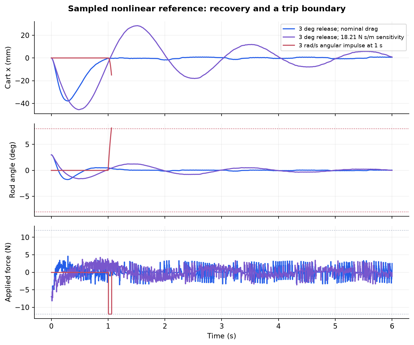
In the nominal nonlinear simulation, a 3-degree release reaches 37.88 mm of cart excursion and 8.154 N peak force. During the last second of a six-second run, cart error stays below 0.851 mm and rod angle below 0.086 degrees. The four tested releases at plus or minus 1 and 3 degrees meet the stated recovery criterion. Those are new numerical predictions, not measurements extracted from the clips.
Show where the reference stops recovering
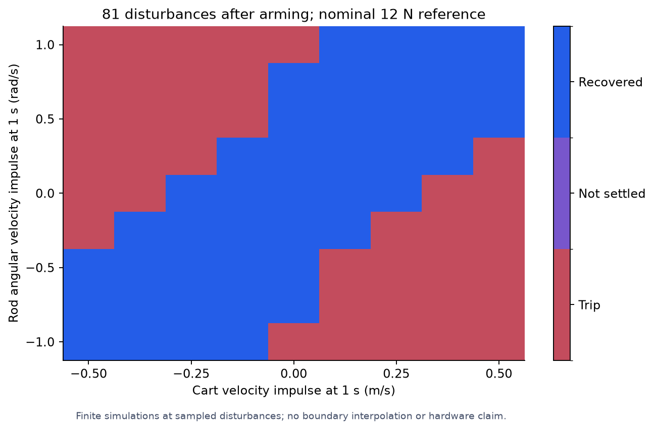
A larger angular-velocity disturbance drives the force into saturation and trips the angle limit. The high-drag sensitivity remains inside the trip limits but misses the six-second position criterion. A finite map of 81 velocity disturbances after arming has 43 recoveries and 38 trips; it is a sampled study rather than a guaranteed stability boundary. Independent solver, energy, linearization and calibration checks support the model within its declared assumptions.
Preserve what the two clips establish
The first clip shows recovery toward upright after small hand-applied disturbances. A larger push is followed by loss of balance in the second. The footage does not isolate whether saturation, travel, estimation or model error caused that failure. It also does not establish a numerical disturbance threshold or identify the original controller timing.
2026 sampled nonlinear reference
2026 finite disturbance study
Project context
2021 Purdue project team. Original hardware footage and calibration are preserved; the 2026 sampled nonlinear reference is separate digital work, with no new physical validation.
Historical photographs, footage, and plots retain their original dates. Later digital reconstructions are identified separately; their numerical checks do not establish hardware performance.